311.2. Filter Transformations

311.2. Filter Transformations¶

For the Rubin Science Platform at data.lsst.cloud.
Data Release: Data Preview 2
Container Size: Large
LSST Science Pipelines version: r30.0.11
Last verified to run: 2026-09-15
Repository: github.com/lsst/tutorial-notebooks
DOI: 10.11578/rubin/dc.20250909.20

Learning objective: An overview of transformation relations to and from the LSSTCam photometric system presented in Data Preview 2 and other commonly-used photometric systems and how to apply these relations.

LSST data products: Object

Packages: lsst.rsp.RSPDiscovery

Credit: Originally developed by the Rubin Community Science team. Please consider acknowledging them if this notebook is used for the preparation of journal articles, software releases, or other notebooks.

Get Support: Everyone is encouraged to ask questions or raise issues in the Support Category of the Rubin Community Forum. Rubin staff will respond to all questions posted there.

1. Introduction¶

Being able to transform measurements between different photometric systems is essential for comparing results with not only contemporaneous and legacy data sets but also with theoretical models (e.g., stellar isochrones) derived using legacy photometric systems.

To this end, the Vera C. Rubin Project has generated transformation relations between the Data Preview 2 (DP2) $ugrizy$ system and other systems, like PanSTARRS1 DR2, Dark Energy Survey (DES) DR2, EUCLID, Gaia DR3, SDSS DR18, and Johnson-Cousins. These transformation relations are provided in Rubin Technical Note 125 (RTN-125).

Two methods for transforming between photometric systems are explored in RTN-125: polynomial relations and lookup tables. The guiding principle for which is to use is driven by the balance between simplicity and accuracy: in general, simple first- or second-order polynomials are sufficient, but, for higher accuracy, one may instead choose the slightly more difficult-to-employ lookup-table method.

This tutorial demonstrates how to apply both methods of photometric transformation. Examples are provided for converting from Rubin DP2 $i$-band photometry to PanSTARRS1 DR2 and DES DR2 $i$ bands, and from Rubin DP2 $g$-band photometry to Gaia DR3 $BP$-band photometry.

Related tutorials: The 100-level tutorials demonstrate how to use the butler, the TAP service, and the Firefly image display. The 200-level tutorials introduce the types of image and catalog data.

1.1. Import packages¶

Import numpy, a fundamental package for scientific computing with arrays in Python (numpy.org), matplotlib, a comprehensive library for data visualization (matplotlib.org; matplotlib gallery), units package (astropy.units), hstack function, Table class, and SkyCoord class from astropy, interpolate module from scipy, and pyvo module for accessing remote data.

From the LSST pacakge (pipelines.lsst.io), import the module for accessing the Table Access Protocol (TAP) service.

In [1]:

import numpy as np
import matplotlib.pyplot as plt
from matplotlib.colors import LogNorm
from astropy import units as u
from astropy.table import hstack, Table
from astropy.coordinates import SkyCoord
from scipy import interpolate
import pyvo

from lsst.rsp import RSPDiscovery

1.2. Define parameters and functions¶

Instantiate RSPDiscovery with the DP2 release, create an instance of the TAP service.

In [2]:

discovery = RSPDiscovery("dp2")
rsp_tap = discovery.get_tap_client()

Define the approximate central coordinates of the ECDFS field and a radius of 0.24 degrees about this center.

Note: The radius is restricted to 0.24 degrees here, since the public PanSTARRS1 DR2 TAP service -- which is used later in this notebook -- is currently restricted to cone searches less than 0.25 degrees.

In [3]:

ra_cen = 53.2
dec_cen = -28.1
radius = 0.24

Define parameters to use colorblind-friendly colors with matplotlib.

In [4]:

plt.style.use('seaborn-v0_8-colorblind')
prop_cycle = plt.rcParams['axes.prop_cycle']
colors = prop_cycle.by_key()['color']

Define a function for cross-matching between sky catalogs.

In [5]:

def cross_match_catalogs(tab1, tab2, ra_name_1, dec_name_1, ra_name_2, dec_name_2, radius_arcsec=3.0):
    """Match two catalogs based on RA, Dec coordinates using Astropy Tables.
    Keep only the closest match in cases where multiple sources in tab1 match the same source in tab2.

    Parameters
    ----------
    tab1, tab2 : `astropy.table.Table`
        The catalogs to be matched.
    ra_name_1, dec_name_1 : `str`
        Column names for right ascension and declination in tab1.
    ra_name_2, dec_name_2 : `str`
        Column names for right ascension and declination in tab2.
    radius_arcsec : `float`, optional
        Maximum separation for a valid match (default is 3.0).

    Returns
    -------
    matches : `astropy.table.Table`
        Table of matched objects (horizontally stacked).
    """
    coords1 = SkyCoord(ra=np.array(tab1[ra_name_1]), dec=np.array(tab1[dec_name_1]), unit=u.degree)
    coords2 = SkyCoord(ra=np.array(tab2[ra_name_2]), dec=np.array(tab2[dec_name_2]), unit=u.degree)

    idx, d2d, _ = coords1.match_to_catalog_sky(coords2)
    mask = d2d < (radius_arcsec * u.arcsec)

    tab1_matched = tab1[mask].copy()
    tab2_matched = tab2[idx[mask]].copy()

    tab1_matched['separation_arcsec'] = d2d[mask].arcsec
    tab1_matched['match_idx'] = idx[mask]

    matches = hstack([tab1_matched, tab2_matched], table_names=['1', '2'])

    matches.sort('separation_arcsec')
    _, unique_indices = np.unique(matches['match_idx'], return_index=True)
    matches = matches[unique_indices]
    matches.remove_column('match_idx')

    return matches

2. Grab LSSTCam ECDFS point source data from DP2¶

Define a query to grab stars in the ECDFS field from the DP2 Object table. To avoid potentially saturated stars and very faint stars, restrict the sample returned to those point sources with $r$-band magnitudes between 16.0 and 24.0.

In [6]:

query = """
        SELECT coord_ra, coord_dec, objectId,
            u_psfMag, g_psfMag, r_psfMag, i_psfMag, z_psfMag,
            u_psfMagErr, g_psfMagErr, r_psfMagErr, i_psfMagErr, z_psfMagErr,
            refExtendedness
        FROM dp2.Object
        WHERE CONTAINS(POINT('ICRS', coord_ra, coord_dec),
            CIRCLE('ICRS', {}, {}, {}))=1
        AND refExtendedness=0
        AND r_psfMag BETWEEN 16.0 AND 24.0
        """.format(ra_cen, dec_cen, radius)

In [7]:

job = rsp_tap.submit_job(query)
job.run()
job.wait(phases=['COMPLETED', 'ERROR'])
print('Job phase is', job.phase)
if job.phase == 'ERROR':
    job.raise_if_error()

Job phase is COMPLETED

Fetch the results and store them as a table.

In [8]:

df_dp2 = job.fetch_result().to_table()
print(f"The query returned {len(df_dp2)} objects.")

The query returned 923 objects.

Option to display the table of results.

In [9]:

# df_dp2

Calculate color indices using the PSF magnitudes, and plot a color-color diagram. Color-code points by the $r$-band PSF magnitude error.

In [10]:

df_dp2['gr_psfMag'] = df_dp2['g_psfMag'] - df_dp2['r_psfMag']
df_dp2['ri_psfMag'] = df_dp2['r_psfMag'] - df_dp2['i_psfMag']
df_dp2['gi_psfMag'] = df_dp2['g_psfMag'] - df_dp2['i_psfMag']

plt.figure(figsize=(10, 6))
sc = plt.scatter(
    df_dp2['gr_psfMag'],
    df_dp2['ri_psfMag'],
    c=df_dp2['r_psfMagErr'],
    cmap='viridis',
    alpha=0.7,
    s=8,
    vmin=0.00,
    vmax=0.02
)

plt.xlabel('g - r')
plt.ylabel('r - i')
plt.title('color-color diagram for 16<r<24 point sources in ECDFS')
plt.grid(True)
plt.xlim(-0.5, 2.0)
plt.ylim(-0.5, 2.5)

cbar = plt.colorbar(sc)
cbar.set_label('r_psfMagErr')

plt.show()

Figure 1: ($r$-$i$) vs. ($g$-$r$) color-color diagram for point sources in a 0.24-degree radius of the ECDFS field in DP2 data. Points are calculated from Object table PSF magnitudes, and are color-coded by their $r$-band PSF magnitude error, ranging from 0 to 0.02 magnitudes. The figure shows the typical stellar locus as a narrow sequence with a sharp upturn at red colors.

3. First-order polynomial transformation: LSSTCam $i$ --> PanSTARRS1 DR2 $i$¶

As a simple first case, look at the polynomial transformation from DP2 $i$-band to PanSTARRS1 DR2 $i$-band.

3.1. Examine the transformation relation¶

Find the section in RTN-125 that describes the polynomial transformation relation between the DP2 and PanSTARRS1 DR2 systems.

Here is the line from RTN-125 that describes the transform from DP2 $i$-band to PanSTARRS1 DR2 $i$-band:

Conversion	Transformation Equation	RMS	Applicable Color Range	QA Plot
$i_{LSST} \to i_{ps1}$	$i_{ps1} - i_{LSST} = +0.007 (g-i)_{LSST} - 0.006$	0.012	$-0.7 < (g-i)_{LSST} \leq 3.7$	link

Here are the quality assurance (QA) plots from RTN-125 associated with the first-order polynomial fit of the DP2 $i$-band to PanSTARRS1 DR2 $i$-band:

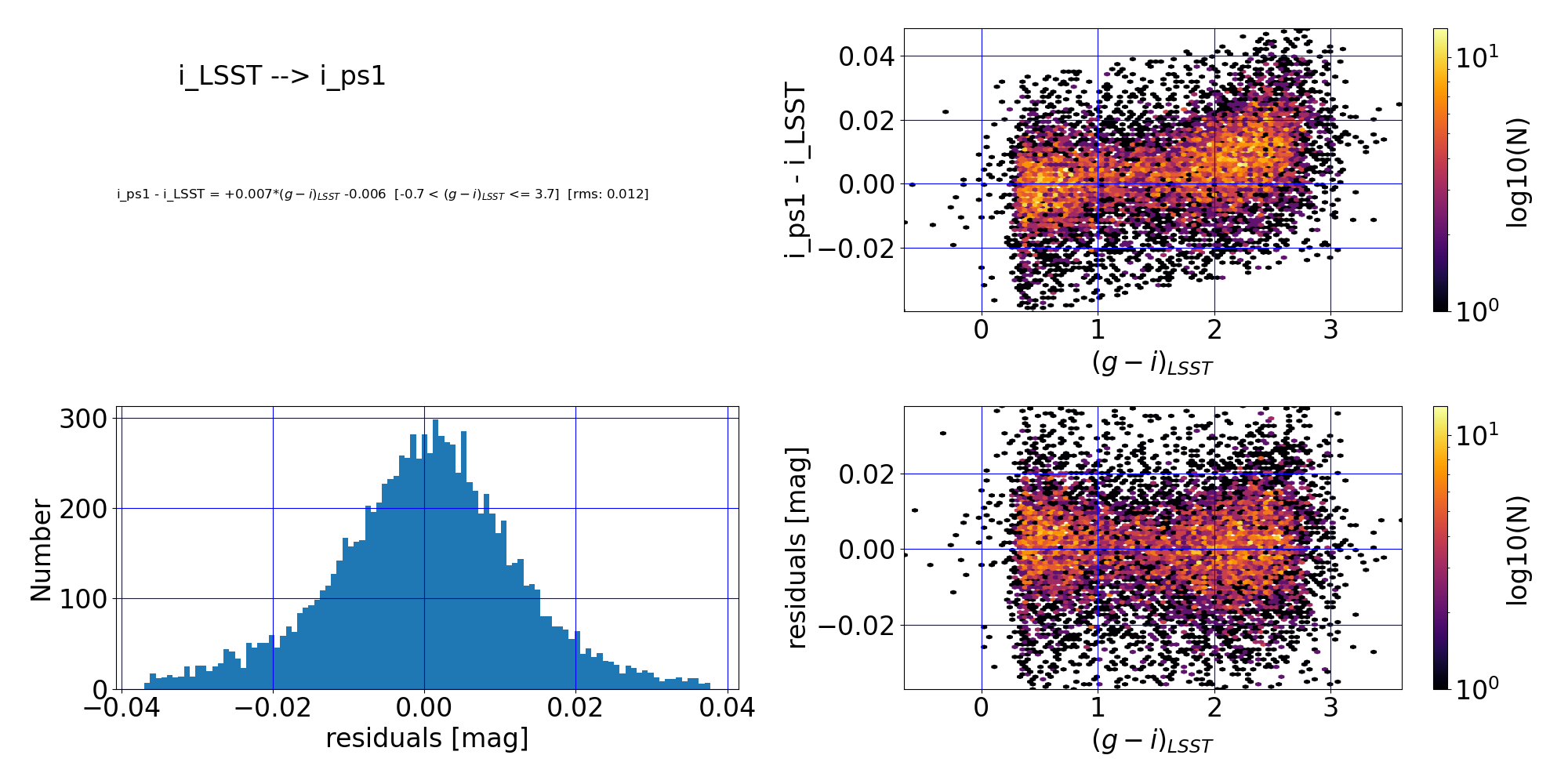
Figure 2: Comparison of LSSTCam DP2 and PS1 DR2 $i$-band photometry. (Top left:) The fit polynomial equation, the RMS of the fit, and the applicable color range. (Top right:) The difference between the two magnitudes vs. color before any transformation. (Bottom left:) Histogram of the residuals of the fit. (Bottom right:) Residuals of the fit vs. ($g$-$i$) color. The residuals scatter about zero, suggesting that the fit has done a reasonable job.

3.2. Apply the transformation¶

Select only stars within the applicable color range (-0.7 < $g-i$ <= 3.7) from the fit. Apply the polynomial transformation to these stars from the LSSTCam data in the ECDFS field.

In [11]:

pick_ps1dr2_colors = (df_dp2['gi_psfMag'] <= 3.7) & (df_dp2['gi_psfMag'] > -0.7)
df_dp2_ps1dr2_transform = df_dp2[pick_ps1dr2_colors].copy()

df_dp2_ps1dr2_transform['i_ps1_poly_offset'] = 0.007*df_dp2_ps1dr2_transform['gi_psfMag'] - 0.006
df_dp2_ps1dr2_transform['i_ps1_poly'] = df_dp2_ps1dr2_transform['i_psfMag'] + df_dp2_ps1dr2_transform['i_ps1_poly_offset']

3.3. Test the transformation¶

Test the transformation by comparing the PS1 $i$-band magnitudes estimated from the DP2 data in ECDFS against the PS1 $i$-band magnitudes from the PanSTARRS1 DR2 data themselves.

3.3.1. Grab ECDFS data from PanSTARRS1 DR2¶

Use pyvo to query the PanSTARRS1 DR2 TAP service, using suitable constraints for point sources. Since the PanSTARRS1 DR2 TAP service has a cone search maximum search radius of 0.25 deg, keep the search to less than that fixed radius.

Note: Safely ignore the DALOverflowWarning regarding truncated results. This is expected behavior for this query and the returned subset is sufficient for this demonstration.

In [12]:

ps1dr2_tap_url = 'https://mast.stsci.edu/vo-tap/api/v0.1/ps1dr2'
ps1dr2_tap = pyvo.dal.TAPService(ps1dr2_tap_url)

query = """
        SELECT o.raMean, o.decMean, o.iMeanPSFMag
        FROM dbo.MeanObjectView o
        LEFT JOIN StackObjectAttributes AS soa ON soa.objID = o.objID
        WHERE CONTAINS(POINT('ICRS', RAMean, DecMean),
            CIRCLE('ICRS', {}, {}, {}))=1
        AND o.nDetections > 5
        AND soa.primaryDetection > 0
        AND o.gQfPerfect > 0.85 and o.rQfPerfect > 0.85 and o.iQfPerfect > 0.85 and o.zQfPerfect > 0.85
        AND (o.rmeanpsfmag - o.rmeankronmag < 0.05)
        """.format(ra_cen, dec_cen, radius)

job = ps1dr2_tap.run_async(query)
df_ps1 = job.to_table()

/opt/lsst/software/stack/conda/envs/lsst-scipipe-12.3.0-exact/lib/python3.13/site-packages/pyvo/dal/query.py:403: DALOverflowWarning: Results truncated due to server limits. Consider setting a maxrec value.
  warn("Results truncated due to server limits. Consider "

3.3.2 Match the ECDFS data from DP2 with the ECDFS data from PanSTARRS1 DR2¶

Use the cross_match_catalogs function defined above to match the two catalogs based on the stars' coordinates.

In [13]:

matches_dp1_ps1 = cross_match_catalogs(df_dp2_ps1dr2_transform, df_ps1,
                                       'coord_ra', 'coord_dec', 'ramean', 'decmean')

3.3.3. Compare the DP2-estimated PS1 i-band magnitudes with the PanSTARRS1 DR2 i-band magnitudes¶

Calculate both the differences between the DP2 $i$-band magnitude and the PanSTARRS1 DR2 $i$-band magnitude ("before transformation") and the differences between DP2-estimated PS1 $i$-band magnitude and the PanSTARRS1 DR2 $i$-band magnitude ("after transformation").

In [14]:

matches_dp1_ps1['dmag_i_cc_ps1'] = matches_dp1_ps1['i_psfMag'] - matches_dp1_ps1['imeanpsfmag']
matches_dp1_ps1['dmag_i_ps1_poly'] = matches_dp1_ps1['i_ps1_poly'] - matches_dp1_ps1['imeanpsfmag']

Plot the histogram of the $\Delta$mags (both before transformation and post transformation).

In [15]:

dmag_orig = matches_dp1_ps1['dmag_i_cc_ps1']
dmag_new = matches_dp1_ps1['dmag_i_ps1_poly']

dmag_min, dmag_max = -0.2, 0.2
n_bins = 10 if len(dmag_new) < 100 else 100

fig, ax = plt.subplots()
ax.hist(dmag_orig, bins=n_bins, range=(dmag_min, dmag_max), color=colors[2],
        alpha=0.50, label='Before transformation')

ax.hist(dmag_new, bins=n_bins, range=(dmag_min, dmag_max), color=colors[5],
        alpha=0.50, label='After transformation')

ax.set_xlabel(r'$\Delta$mag [mag]')
ax.set_ylabel('Number')
ax.set_title(r'Difference between DP2 and PanSTARRS1 DR2 $i$-band')

ax.grid(True, color='grey', alpha=0.3, linestyle='--')
ax.legend()

plt.show()

Figure 3: Histogram comparing DP2 and PS1 DR2 $i$-band photometry for matched stars; differences are calculated as $\Delta$mag = DP2 mag - PS1 mag. The orange histogram shows the difference before applying the transformation, demonstrating that there is a tail to negative $\Delta$mag values. The blue histogram is the result after applying the polynomial transformation. The transformed difference is centered on a magnitude residual of zero, as expected.

Create a scatter plot of the $\Delta$mags (both before transformation and post transformation) vs. color. Note that LSSTCam DP2 $i$-band and PanSTARRS1 DR2 $i$-band are fairly similar; so the transformation is relatively small.

In [16]:

color = matches_dp1_ps1['gi_psfMag']
color_min, color_max = -0.7, 3.7
dmag_min, dmag_max = -0.1, 0.3

fig, ax = plt.subplots()
ax.scatter(color, dmag_orig, color=colors[2], alpha=0.50,
           label='Before transformation')
ax.scatter(color, dmag_new, color=colors[5], alpha=0.50, marker='*',
           label='After transformation')

ax.axhline(0, color='black', linestyle=':', alpha=0.7)
ax.set_xlim(color_min, color_max)
ax.set_ylim(dmag_min, dmag_max)
ax.set_xlabel(r'$(g-i)_{\mathrm{LSST}}$')
ax.set_ylabel(r'$\Delta$mag [mag]')
ax.set_title(r'$\Delta$mag between DP2 and PanSTARRS1 DR2 $i$-band vs. $(g-i)$')

ax.grid(True, color='grey', alpha=0.3, linestyle='--')
ax.legend()

plt.show()

Figure 4: Magnitude differences between LSSTCam DP2 and PS1 DR2 $i$-band photometry for matched stars plotted as a function of $(g-i)$ color. Orange points show the difference before applying the transformation. Blue stars are the results after applying the polynomial transformation. The transformed difference is centered on a magnitude residual of zero, as expected.

4. Piecewise 1st-order polynomial transformation: DP2 $i$ --> DES DR2 $i$¶

Now look at the polynomial transformation from DP2 $i$-band to DES DR2 $i$-band. This is a little more complicated than the previous example, as there is a break in the relation; so this polynomial had to be fit piece-wise, with a break at $(g-i)_{LSST} = 1.8$.

4.1. Examine the transformation relation¶

Find the section in RTN-125 that describes the polynomial transformation relation between the DP2 system and the DES DR2 system.

Here are the lines from RTN-125 that describes the transform from DP2 $i$-band to DES DR2 $i$-band:

Conversion	Transformation Equation	RMS	Applicable Color Range	QA Plot
$i_{LSST} \to i_{des}$	$i_{des} - i_{LSST} = -0.049 (g-i)_{LSST} + 0.018$	0.010	$-0.8 < (g-i)_{LSST} \leq 1.8$	link
$i_{LSST} \to i_{des}$	$i_{des} - i_{LSST} = -0.121 (g-i)_{LSST} + 0.144$	0.012	$1.8 < (g-i)_{LSST} \leq 3.8$	link

Here are the QA plots from RTN-125 associated with the first-order piece-wise polynomial fit of the DP2 $i$-band to DES DR2 $i$-band:

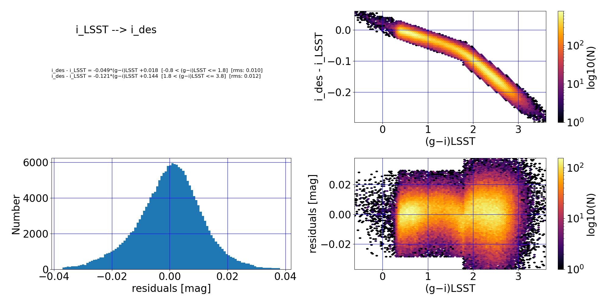
Figure 5: Comparison of LSSTCam DP2 and DES DR2 $i$-band photometry. (Top left:) The fit polynomial equation, the RMS of the fit, and the applicable color range. (Top right:) The difference between the two magnitudes vs. color before any transformation. (Bottom left:) Histogram of the residuals of the fit. (Bottom right:) Residuals of the fit vs. ($g$-$i$) color. The residuals scatter about zero, suggesting that the fit has done a reasonable job.

4.2. Apply the transformation¶

Apply the transformation to the LSSTCam DP2 data in the ECDFS field. This requires first defining the two color ranges in which to apply the separate piece-wise components.

In [17]:

condlist = [
    (df_dp2['gi_psfMag'] > -0.8) & (df_dp2['gi_psfMag'] <= 1.8),
    (df_dp2['gi_psfMag'] > 1.8) & (df_dp2['gi_psfMag'] <= 3.8)]

choicelist = [
    -0.049 * df_dp2['gi_psfMag'] + 0.018,
    -0.121 * df_dp2['gi_psfMag'] + 0.144]

df_dp2['i_des_poly_offset'] = np.select(condlist, choicelist, default=np.nan)
df_dp2['i_des_poly'] = df_dp2['i_psfMag'] + df_dp2['i_des_poly_offset']

4.3. Test the transformation¶

Test the transformation by comparing the DES $i$-band magnitudes estimated from the DP2 data in ECDFS against the DES $i$-band magnitudes from the DES DR2 data themselves.

4.3.1. Grab ECDFS data from DES DR2¶

Query the NOIRLab Astro Data Lab TAP service for the DES DR2 data, using suitable constraints for point sources. Note that ADQL cone search does not seem to work for DES DR2; so ranges in ra and dec are used instead.

In [18]:

tap_service = pyvo.dal.TAPService("https://datalab.noirlab.edu/tap")

ra_offset = radius / np.cos(np.radians(dec_cen))
ra_min = ra_cen - ra_offset
ra_max = ra_cen + ra_offset
dec_min = dec_cen - radius
dec_max = dec_cen + radius

query = """
        SELECT ra, dec, WAVG_MAG_PSF_I
        FROM des_dr2.main
        WHERE (ra BETWEEN {} AND {})
        AND (dec BETWEEN {} AND {})
        AND (WAVG_MAGERR_PSF_R BETWEEN 0.00 AND 0.05) AND (WAVG_MAG_PSF_R < 24.0)
        AND (EXTENDED_CLASS_WAVG = 0)
        AND (FLAGS_G < 4 AND FLAGS_R < 4 AND FLAGS_I < 4)
        """.format(ra_min, ra_max, dec_min, dec_max)

results = tap_service.search(query)
df_desdr2 = results.to_table()

4.3.2. Match the ECDFS data from DP2 with the ECDFS data from DES DR2¶

Use the cross_match_catalogs function to match the two catalogs.

In [19]:

matches_dp2_desdr2 = cross_match_catalogs(df_dp2, df_desdr2,
                                          'coord_ra', 'coord_dec', 'ra', 'dec')

4.3.3. Compare the DP2-estimated PS1 i-band magnitudes with the DES DR2 i-band magnitudes¶

Calculate both the differences between the DP2 $i$-band magnitude and the DES DR2 $i$-band magnitude ("before transformation") and the differences between DP2-estimated DES $i$-band magnitude and the DES DR2 $i$-band magnitude ("after transformation").

In [20]:

matches_dp2_desdr2['dmag_i_cc_des'] = matches_dp2_desdr2['i_psfMag'] - matches_dp2_desdr2['wavg_mag_psf_i']
matches_dp2_desdr2['dmag_i_des_poly'] = matches_dp2_desdr2['i_des_poly'] - matches_dp2_desdr2['wavg_mag_psf_i']

Plot the histogram of the $\Delta$mags (both before transformation and post transformation).

In [21]:

dmag_orig = matches_dp2_desdr2['dmag_i_cc_des']
dmag_new = matches_dp2_desdr2['dmag_i_des_poly']

dmag_min, dmag_max = -0.3, 0.3
n_bins = 10 if len(dmag_new) < 100 else 100

fig, ax = plt.subplots()
ax.hist(dmag_orig, bins=n_bins, range=(dmag_min, dmag_max), color=colors[2],
        alpha=0.50, label='Before transformation')

ax.hist(dmag_new, bins=n_bins, range=(dmag_min, dmag_max), color=colors[5],
        alpha=0.50, label='After transformation')

ax.set_xlabel(r'$\Delta$mag [mag]')
ax.set_ylabel('Number')
ax.set_title(r'Difference between DP2 and DES DR2 $i$-band')

ax.grid(True, color='grey', alpha=0.3, linestyle='--')
ax.legend()

plt.show()

Figure 6: Histogram comparing LSSTCam DP2 and DES DR2 $i$-band photometry for matched stars; differences are calculated as $\Delta$mag = DP2 mag - DES mag. The orange histogram shows the difference before applying the transformation, demonstrating that there is a significant offset in $\Delta$mag values to positive residuals. The blue histogram is the result after applying the polynomial transformation. The transformed difference is centered on a magnitude residual of zero, as expected.

Create a scatter plot of the $\Delta$mags (both before transformation and post transformation) vs. color. Note that the DES DR2 $i$-band differs more from the LSSTCam DP2 $i$-band than does the PanSTARRS1 DR2 $i$-band; so the transformation is larger than in the previous example.

In [22]:

color = matches_dp2_desdr2['gi_psfMag']
color_min, color_max = -0.8, 3.8
dmag_min, dmag_max = -0.3, 0.3

fig, ax = plt.subplots()
ax.scatter(color, dmag_orig, color=colors[2], alpha=0.50,
           label='Before transformation')
ax.scatter(color, dmag_new, color=colors[5], alpha=0.50, marker='*',
           label='After transformation')

ax.axhline(0, color='black', linestyle=':', alpha=0.7)
ax.set_xlim(color_min, color_max)
ax.set_ylim(dmag_min, dmag_max)
ax.set_xlabel(r'$(g-i)_{\mathrm{LSST}}$')
ax.set_ylabel(r'$\Delta$mag [mag]')
ax.set_title(r'$\Delta$mag between DP2 and DES DR2 $i$-band vs. $(g-i)$')

ax.grid(True, color='grey', alpha=0.3, linestyle='--')
ax.legend()

plt.show()

Figure 7: Magnitude differences between DP2 and DES DR2 $i$-band photometry for matched stars plotted as a function of $(g-i)$ color. Orange points show the difference before applying the transformation, demonstrating a large offset in $\Delta$mag that increases at redder $(g-i)$ colors. Blue stars are the results after applying the polynomial transformation. The transformed difference is centered on a magnitude residual of zero, as expected.

5. Second-order polynomial transformation: LSSTCam $g$ --> Gaia DR3 $BP_{gaia}$¶

Next, look at the polynomial transformation from DP2 $g$-band to Gaia DR3 $BP$-band. Here, a first-order polynomial fit is insufficient, so a second-order polynomial fit is employed. One could consider even higher terms to achieve a more accurate relation, but that is left to the lookup table transformation method described in the next section.

5.1. Examine the transformation relation¶

Find the section in RTN-125 that describes the polynomial transformation relation between the DP2 system and the Gaia DR3 system.

Here are the lines from RTN-125 that describe the transform from DP2 $g$-band to Gaia DR3 $BP$-band:

Conversion	Transformation Equation	RMS	Applicable Color Range	QA Plot
$g_{LSST} \to BP_{gaia}$	$BP_{gaia} - g_{LSST} = +0.096 (g-i)_{LSST}^2 - 0.487 (g-i)_{LSST} + 0.194$	0.037	$0.3 < (g-i)_{LSST} \leq 3.2$	link

Here are the QA plots from RTN-125 associated with the second-order polynomial fit of the DP2 $g$-band to Gaia DR3 $BP$-band. Note from the bottom-right plot that a third-order term might benefit the fit, but staying with the simpler second-order polynomial still achieves a 0.037 mag RMS in the fit. For more accuracy, using the lookup table method (described in the next section) is recommended.

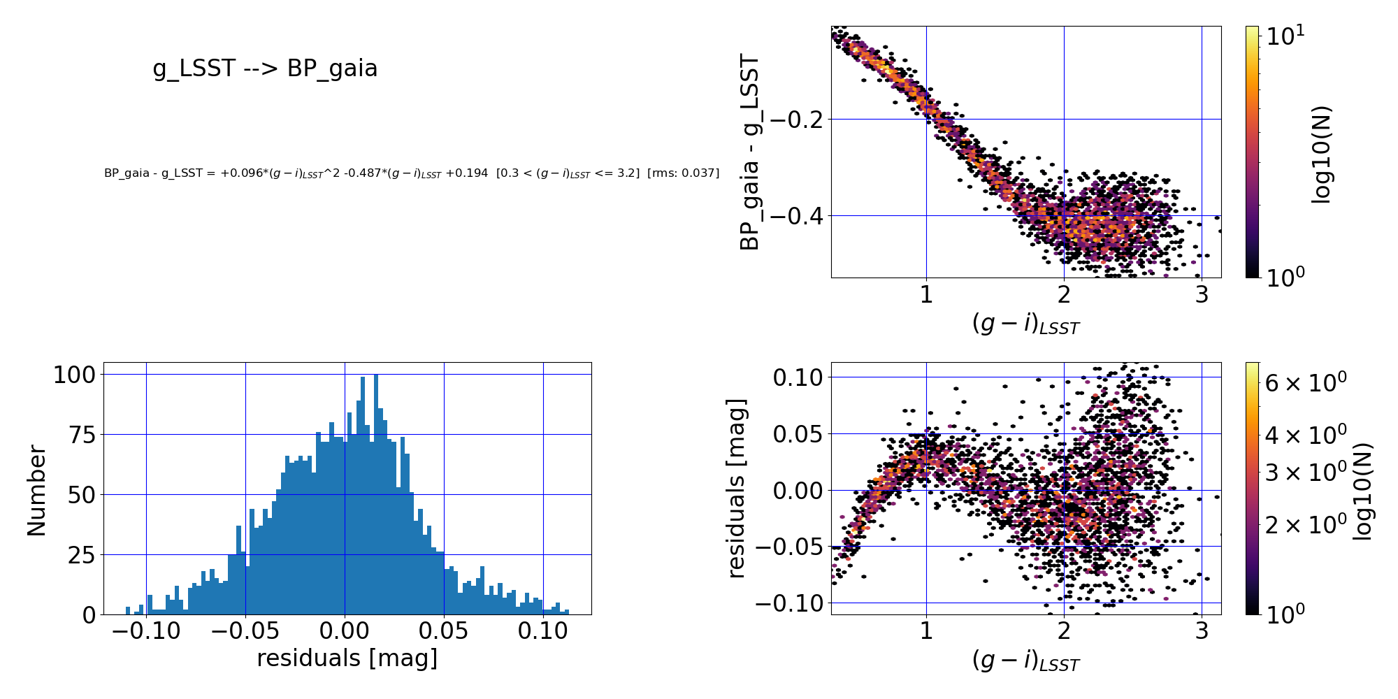
Figure 8: Comparison of LSSTCam DP2 $g$-band and Gaia DR3 $BP$-band photometry. (Top left:) The fit polynomial equation, the RMS of the fit, and the applicable color range. (Top right:) The difference between the two magnitudes vs. color before any transformation. (Bottom left:) Histogram of the residuals of the fit. (Bottom right:) Residuals of the fit vs. ($g$-$i$) color. The residuals scatter about zero, suggesting that the fit has done a reasonable job, though there is a clear pattern remaining that could be mitigated by using a higher-order fit.

5.2. Apply the transformation¶

Select only stars within the applicable color range (0.3 < $g-i$ <= 3.2) from the fit. Apply the polynomial transformation to these stars from the DP2 data in the ECDFS field.

In [23]:

pick_gaia_colors = (df_dp2['gi_psfMag'] <= 3.2) & (df_dp2['gi_psfMag'] > 0.3)
df_dp2_gaia_transform = df_dp2[pick_gaia_colors].copy()

df_dp2_gaia_transform['BP_gaia_poly_offset'] = 0.096*np.pow(df_dp2_gaia_transform['gi_psfMag'], 2.) -\
                                               0.487*df_dp2_gaia_transform['gi_psfMag'] + 0.194
df_dp2_gaia_transform['BP_gaia_poly'] = df_dp2_gaia_transform['g_psfMag'] + df_dp2_gaia_transform['BP_gaia_poly_offset']

5.3. Test the transformation¶

Test the transformation by comparing the Gaia DR3 $BP$-band magnitudes estimated from the DP2 data in ECDFS against the Gaia DR3 $BP$-band magnitudes from the Gaia DR3 data themselves in ECDFS.

5.3.1. Grab ECDFS data from Gaia DR3¶

Query the Gaia DR3 TAP service, using suitable constraints for a clean sample.

In [24]:

gaia_tap_url = 'https://gaia.aip.de/tap'
gaia_tap = pyvo.dal.TAPService(gaia_tap_url)

query = """
        SELECT ra, dec, phot_bp_mean_mag, phot_g_mean_mag
        FROM gaiadr3.gaia_source_lite
        WHERE
            CONTAINS(POINT('ICRS', ra, dec), CIRCLE('ICRS', {}, {}, {}))=1
        AND parallax_over_error > 5
        AND ruwe < 1.4
        AND phot_g_mean_flux_over_error > 5
        AND phot_rp_mean_flux_over_error > 5
        AND phot_bp_mean_flux_over_error > 5
        """.format(ra_cen, dec_cen, radius)

result = gaia_tap.run_sync(query)
df_gaiadr3 = result.to_table()

5.3.2. Match the ECDFS data from DP2 with the ECDFS data from Gaia DR3¶

Use the cross_match_catalogs function to match the two catalogs.

In [25]:

matches_dp2_gaiadr3 = cross_match_catalogs(df_dp2_gaia_transform, df_gaiadr3,
                                           'coord_ra', 'coord_dec', 'ra', 'dec')

5.3.3. Compare the DP2-estimated BP magnitudes with the Gaia DR3 BP magnitudes¶

Calculate both the differences between the DP2 $g$-band magnitude and the Gaia DR3 $BP$-band magnitude ("before transformation") and the differences between DP2-estimated Gaia DR3 $BP$-band magnitude and the actual Gaia DR3 $BP$-band magnitude ("after transformation").

In [26]:

matches_dp2_gaiadr3['dmag_g_cc_BP_gaia'] = matches_dp2_gaiadr3['g_psfMag'] - matches_dp2_gaiadr3['phot_bp_mean_mag']
matches_dp2_gaiadr3['dmag_BP_poly'] = matches_dp2_gaiadr3['BP_gaia_poly'] - matches_dp2_gaiadr3['phot_bp_mean_mag']

Plot the histogram of the $\Delta$mags (both before transformation and post transformation).

In [27]:

dmag_orig = matches_dp2_gaiadr3['dmag_g_cc_BP_gaia']
dmag_new = matches_dp2_gaiadr3['dmag_BP_poly']

dmag_min, dmag_max = -0.5, 0.95
n_bins = 10 if len(dmag_new) < 100 else 100

fig, ax = plt.subplots()
ax.hist(dmag_orig, bins=n_bins, range=(dmag_min, dmag_max), color=colors[2],
        alpha=0.50, label='Before transformation')

ax.hist(dmag_new, bins=n_bins, range=(dmag_min, dmag_max), color=colors[5],
        alpha=0.50, label='After transformation')

ax.set_xlabel(r'$\Delta$mag [mag]')
ax.set_ylabel('Number')
ax.set_title(r'Difference between DP2 $g$-band and Gaia DR3 $BP$-band')

ax.grid(True, color='grey', alpha=0.3, linestyle='--')
ax.legend()

plt.show()

Figure 9: Histogram comparing DP2 $g$-band and Gaia DR3 $BP$-band photometry for matched stars; differences are calculated as $\Delta$mag = DP1 mag - Gaia mag. The orange histogram shows the difference between DP2 $g$ magnitudes and Gaia $BP$ magnitudes before applying the transformation, demonstrating that there is a significant offset in $\Delta$mag values to positive residuals. The blue histogram is the result after applying the polynomial transformation to convert DP2 $g$ magnitudes to Gaia $BP$. The transformed difference is centered on a magnitude residual of zero, as expected.

Create a scatter plot of the $\Delta$mags (both before transformation and post transformation) vs. color. Note that the Gaia DR3 $BP$-band differs substantially from the LSSTCam DP2 $g$-band; so the transformation is fairly large.

In [28]:

color = matches_dp2_gaiadr3['gi_psfMag']
color_min, color_max = 0.3, 3.2
dmag_min, dmag_max = -0.5, 1.0

fig, ax = plt.subplots()
ax.scatter(color, dmag_orig, color=colors[2], alpha=0.50,
           label='Before transformation')
ax.scatter(color, dmag_new, color=colors[5], alpha=0.50, marker='*',
           label='After transformation')

ax.axhline(0, color='black', linestyle=':', alpha=0.7)
ax.set_xlim(color_min, color_max)
ax.set_ylim(dmag_min, dmag_max)
ax.set_xlabel(r'$(g-i)_{\mathrm{LSST}}$')
ax.set_ylabel(r'$\Delta$mag [mag]')
ax.set_title(r'$\Delta$mag between DP2 $g$-band (and transformed $BP$-band) and Gaia DR3 $BP$-band vs. $(g-i)$')

ax.grid(True, color='grey', alpha=0.3, linestyle='--')
ax.legend()

plt.show()

Figure 10: Magnitude differences between DP2 $g$-band and Gaia DR3 $BP$-band photometry for matched stars plotted as a function of $(g-i)$ color. Orange points show the difference between DP2 $g$-band magnitudes and Gaia $BP$-band magnitudes before applying the transformation, demonstrating a large offset in $\Delta$mag that increases toward redder $(g-i)$ colors. Blue stars are the results after applying the polynomial transformation. The transformed difference is centered on a magnitude residual of zero, as expected.

6. Lookup table transformation: LSSTCam $r$ --> Gaia DR3 $G_{gaia}$¶

Next, look at the lookup table transformation from DP2 $r$-band to Gaia DR3 $G$-band.

6.1. Examine the transformation relation¶

Find the section in RTN-125 that describes the lookup table relation between the DP2 system and the Gaia DR3 system.

Here is the line from RTN-125 that describes the lookup table transformation from DP2 $r$-band to Gaia DR3 $G$-band:

Conversion	RMS	Applicable Color Range	QA Plot	Lookup Table
$r_{LSST} \to G_{gaia}$	0.02	$0.3 < (g-i)_{LSST} < 2.9$	link	link

Here are the QA plots from RTN-125 that document the lookup‑table transformation from the DP2 $r$‑band to the Gaia DR3 $G$‑band. The lookup table is constructed by binning matched stars in the ECDFS field by their Rubin DP2 $(g–i)$ color, and then tabulating the median magnitude offset between the Gaia DR3 $G$‑band and the DP2 $r$‑band for the stars in each color bin.

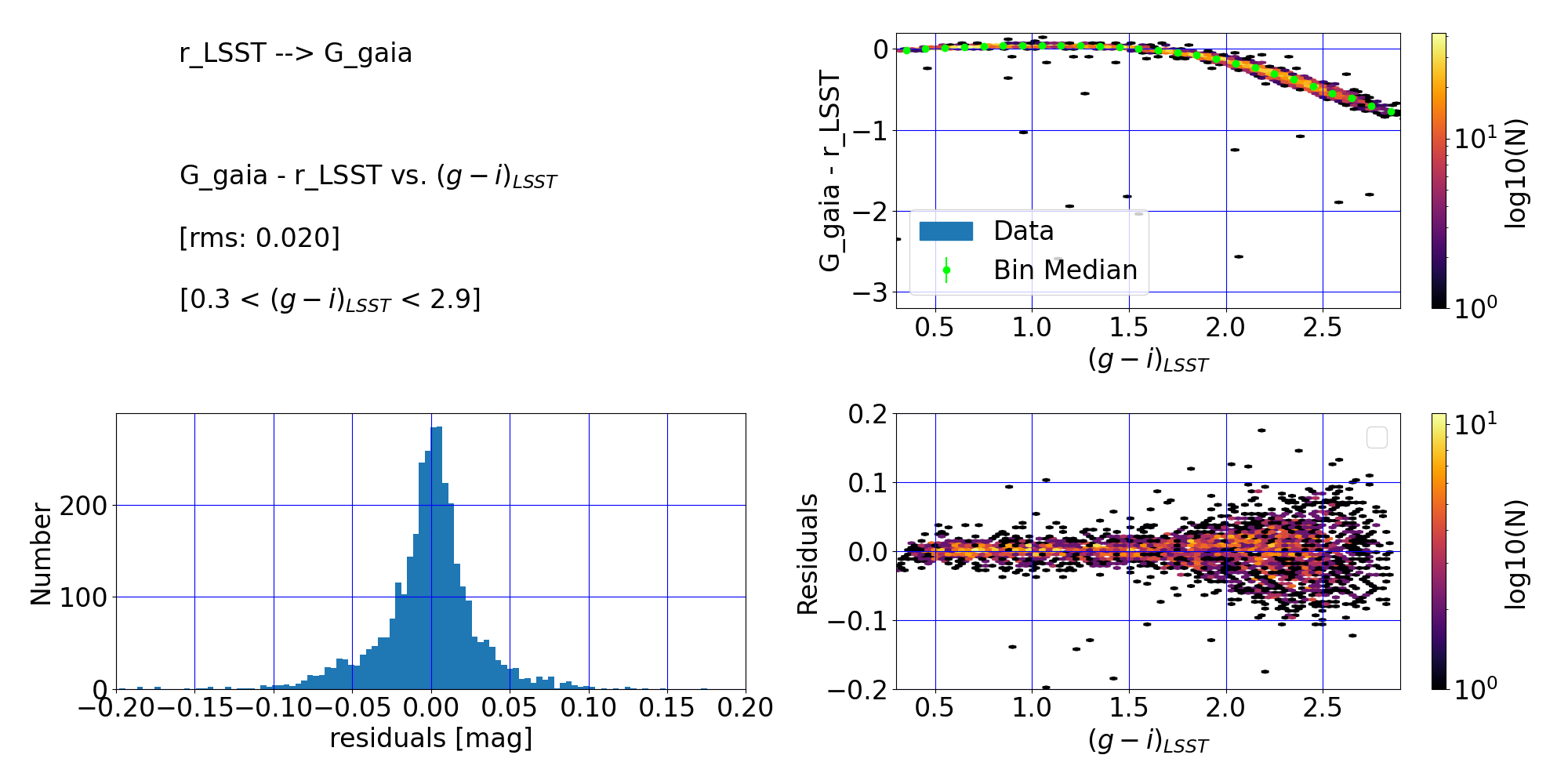
Figure 11: Comparison of DP2 $r$-band and Gaia DR3 $G$-band photometry. (Top left:) The RMS of the linearly interpolated lookup table relation, and the applicable color range. (Top right:) The difference between the two magnitudes vs. color before any transformation. (Bottom left:) Histogram of the residuals from the interpolated lookup table relation. (Bottom right:) Residuals of the interpolated lookup table relation vs. ($g-i$) color. The residuals scatter about zero, suggesting that the fit has done a reasonable job, and the clear pattern remaining after the polynomial fit in Figure 8 has been removed.

6.2. Apply the transformation¶

Copy the URL of the lookup table link from the RTN-125 line in Section 6.1 and assign it to the variable lut_url.

In [29]:

lut_url = "https://rtn-125.lsst.io/_downloads/7b3b7c88167ad2d205e324d2bdd96670/transInterp.LSST_DR2_to_GaiaDR3.G_gaia_gi_LSST.csv"

Read the lookup table, and then display its contents (optional).

In [30]:

lut = Table.read(lut_url, format='ascii.csv')
# lut

Create a 1-d linear interpolation of the median magnitude offset (bin_median) vs. the midpoint of the DP1 $(g-i)$-color bin (bin_label).

In [31]:

response = interpolate.interp1d(lut['bin_label'].astype(float), lut['bin_median'],
                                bounds_error=False, fill_value=0.0, kind='linear')

Calculate and apply the offsets derived from the lookup table.

In [32]:

df_dp2_gaia_transform['G_gaia_lut_offset'] = response(df_dp2_gaia_transform['gi_psfMag'].compressed())
df_dp2_gaia_transform['G_gaia_lut'] = df_dp2_gaia_transform['r_psfMag'] + df_dp2_gaia_transform['G_gaia_lut_offset']

6.3. Test the transformation¶

Test the transformation by comparing the Gaia DR3 $G$-band magnitudes estimated from the DP2 data in ECDFS against the Gaia DR3 $G$-band magnitudes from the Gaia DR3 data themselves.

6.3.1. Match the ECDFS data from DP2 with the ECDFS data from Gaia DR3¶

We re-do this step, as df_dp2 has additional information now.

In [33]:

matches_dp2_gaiadr3 = cross_match_catalogs(df_dp2_gaia_transform, df_gaiadr3,
                                           'coord_ra', 'coord_dec', 'ra', 'dec')

6.3.2. Compare the DP2-estimated G_gaia magnitudes with the Gaia DR3 G_gaia magnitudes¶

Calculate both the differences between the DP2 $r$-band magnitude and the Gaia DR3 $G$-band magnitude ("before transformation") and the differences between DP2-estimated Gaia DR3 $G$-band magnitude and the actual Gaia DR3 $G$-band magnitude ("after transformation").

In [34]:

matches_dp2_gaiadr3['dmag_r_cc_G_gaia'] = matches_dp2_gaiadr3['r_psfMag'] - matches_dp2_gaiadr3['phot_g_mean_mag']
matches_dp2_gaiadr3['dmag_G_lut'] = matches_dp2_gaiadr3['G_gaia_lut'] - matches_dp2_gaiadr3['phot_g_mean_mag']

Plot the histogram of the $\Delta$mags before transformation and after the lookup-table-based transformation.

In [35]:

dmag_orig = matches_dp2_gaiadr3['dmag_r_cc_G_gaia']
dmag_new = matches_dp2_gaiadr3['dmag_G_lut']

dmag_min, dmag_max = -0.2, 0.7
n_bins = 10 if len(dmag_new) < 100 else 100

fig, ax = plt.subplots()
ax.hist(dmag_orig, bins=n_bins, range=(dmag_min, dmag_max), color=colors[2],
        alpha=0.50, label='Before transformation')

ax.hist(dmag_new, bins=n_bins, range=(dmag_min, dmag_max), color=colors[5],
        alpha=0.50, label='After transformation')

ax.set_xlabel(r'$\Delta$mag [mag]')
ax.set_ylabel('Number')
ax.set_title(r'Difference between DP2 $r$-band and Gaia DR3 $G$-band')

ax.grid(True, color='grey', alpha=0.3, linestyle='--')
ax.legend()

plt.show()

Figure 12: Histogram comparing DP2 $r$-band and Gaia DR3 $G$-band photometry for matched stars; differences are calculated as $\Delta$mag = DP2 mag - Gaia mag. The orange histogram shows the difference between DP2 $r$ magnitudes and Gaia $G$ magnitudes before applying the transformation, demonstrating that there is a significant offset in $\Delta$mag values to positive residuals. The blue histogram shows the result after applying the lookup table correction, providing an even narrower distribution about zero net residual.

Create a scatter plot of the $\Delta$mags vs. color for before transformation, and for after the lookup-table-based transformation.

In [36]:

color = matches_dp2_gaiadr3['gi_psfMag']

color_min, color_max = 0.3, 2.9
dmag_min, dmag_max = -0.5, 1.0

fig, ax = plt.subplots()
ax.scatter(color, dmag_orig, color=colors[2], alpha=0.50,
           label='Before transformation')
ax.scatter(color, dmag_new, color=colors[5], alpha=0.50, marker='*',
           label='After transformation')

ax.axhline(0, color='black', linestyle=':', alpha=0.7)
ax.set_xlim(color_min, color_max)
ax.set_ylim(dmag_min, dmag_max)
ax.set_xlabel(r'$(g-i)_{\mathrm{LSST}}$')
ax.set_ylabel(r'$\Delta$mag [mag]')
ax.set_title(r'$\Delta$mag between DP2 $r$-band (and transformed $G$-band) and Gaia DR3 $G$-band vs. $(g-i)$')

ax.grid(True, color='grey', alpha=0.3, linestyle='--')
ax.legend()

plt.show()

Figure 13: Magnitude differences between LSSTComCam $r$-band and Gaia DR3 $G$-band photometry for matched stars plotted as a function of $(g-i)$ color. Orange points show the difference between DP2 $r$ magnitudes and Gaia $G$ magnitudes before applying the transformation, demonstrating a large offset in $\Delta$mag that increases toward redder $(g-i)$ colors. Blue stars show the residuals after transforming using the lookup table, demonstrating smaller residuals.

In [ ]: