102.3. Query for images with ObsTAP

For the Portal Aspect of the Rubin Science Platform (RSP) at data.lsst.cloud.

Data Release: Data Preview 2

Last verified to run: 2026-09-07

Learning objective: Use the ObsTAP service (the ivoa.ObsCore image metadata table) to set up and execute an image query with the Portal’s graphical user interface (UI), without writing ADQL.

LSST data products: deep_coadd

Credit: Originally developed by the Rubin Community Science team. Please consider acknowledging them if this tutorial is used for the preparation of journal articles, software releases, or other tutorials. DOI: 10.11578/rubin/dc.20250909.20

Get Support: Everyone is encouraged to ask questions or raise issues in the Support Category of the Rubin Community Forum. Rubin staff will respond to all questions posted there.

---

Note

Early Data Preview 2 provides deep_coadd images only. Visit, difference, and template images are added with the full DP2 release; once available, the same ObsTAP interface can be used to query for them by selecting the corresponding calibration level and data product subtype.

1. Go to the RSP and enter the Portal Aspect. In a web browser, go to data.lsst.cloud, click on the “Portal” panel, and log in.

2. Open the image search interface. Click on the tab labeled “DP1 & DP2 Images”. The same interface is also reached from the “DP1 & DP2 Catalogs” tab by switching on the “Use Image Search (ObsTAP)” toggle, which selects the ivoa.ObsCore table.

3. Mouse-over for pop-up notes. In the “DP1 & DP2 Images” tab (Figure 1) hover over the components of the UI, or click on the question marks, to see pop-up explanations of the functionality.

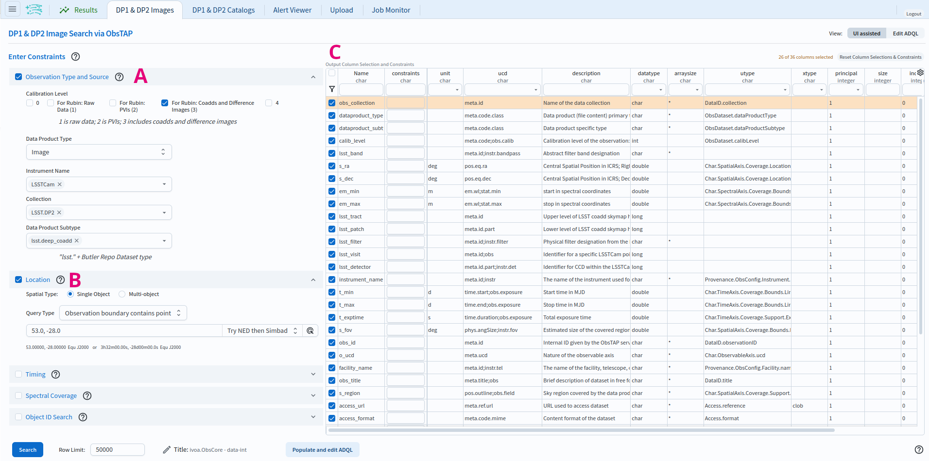
Figure 1: The Portal user interface (UI) for querying images with ObsTAP.

4. Review the UI components. In the Portal UI (Figure 1) review the main components labeled A through C, which are used together to query (search) and retrieve images.

• A: “Observation Type and Source” panel. Set the calibration level, data product type, instrument, collection, and data product subtype, to choose which image product is returned.

• B: “Location” panel. Set the spatial constraint. The “Query Type” drop-down chooses how the region relates to each image’s footprint (e.g., “Observation boundary contains point”).

• C: The ivoa.ObsCore table holds all image metadata. It is recommended to use all pre-selected columns.

The “Timing” and “Spectral Coverage” panels below “Location” add optional temporal and band constraints; neither is used here, as a time constraint does not apply to coadds, which combine many epochs.

5. Set the observation type and source. Expand the “Observation Type and Source” panel. Set the calibration level to “For Rubin: Coadds and Difference Images (3)”, the data product type to “Image”, the instrument name to “LSSTCam”, the collection to “LSST.DP2”, and the data product subtype to “lsst.deep_coadd”.

6. Set the location. Expand the “Location” panel. Set “Spatial Type” to “Single Object” and “Query Type” to “Observation boundary contains point”, and enter 53, -28 (the approximate center of the ECDFS field) in the coordinates field.

7. Execute the search. Click on the “Search” button at lower left.

8. Review the results. The results interface enables interactive visualization of the six deep_coadd images which meet the search criteria: the u, g, r, i, z, y coadds of the single ECDFS patch whose footprint contains the target point.

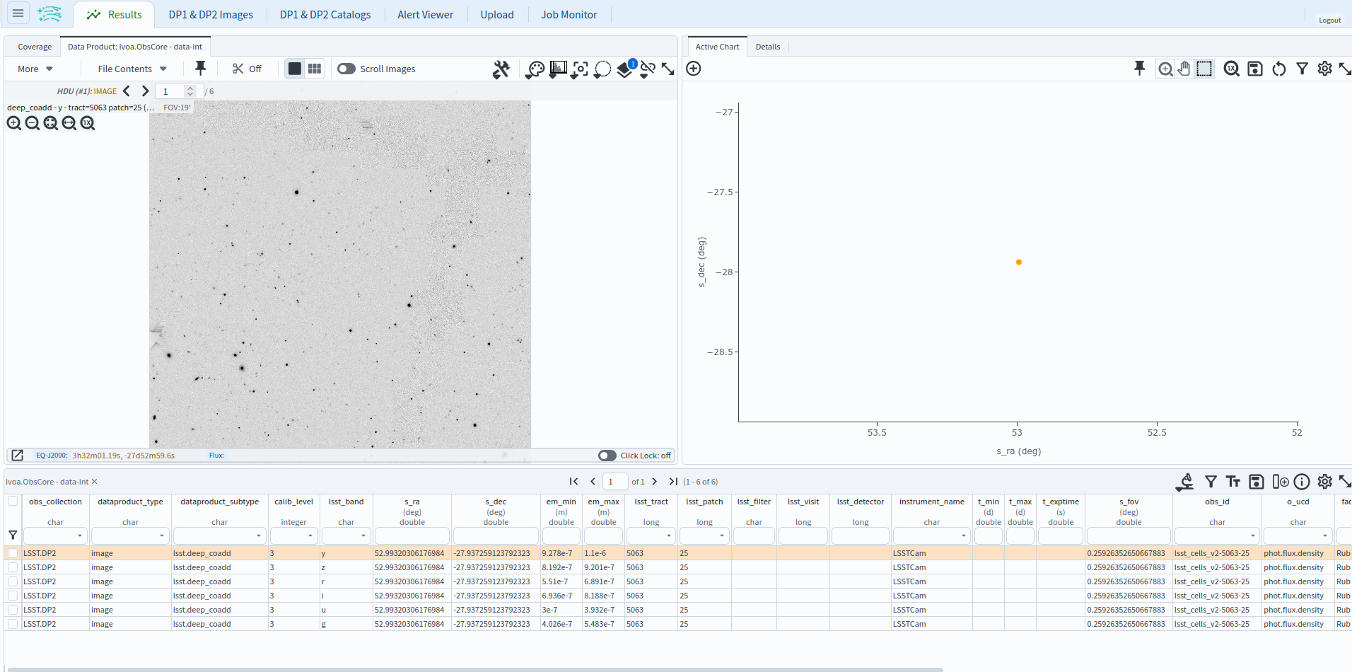
Figure 2: The image results interface, showing the six deep_coadd images (one per band) that meet the search criteria.

Next steps: Tutorial 102.2 performs a similar image query with the SIAv2 service instead of ObsTAP, Tutorial 103.4 writes the equivalent ObsTAP query directly in ADQL, and the 105-series tutorials show how to work with image results in the Firefly viewer.