302.1. PSF photometry for stars

For the Portal Aspect of the Rubin Science Platform at data.lsst.cloud.

Data Release: DP2

Last verified to run: 2026-11-05

Learning objective: To understand the Point Spread Function (PSF) photometry for stars.

LSST data products: Object

Credit: Originally developed by the Rubin Community Science team. Please consider acknowledging them if this tutorial is used for the preparation of journal articles, software releases, or other tutorials. DOI: 10.11578/rubin/dc.20250909.20

Get Support: Everyone is encouraged to ask questions or raise issues in the Support Category of the Rubin Community Forum. Rubin staff will respond to all questions posted there.

---

1. Execute an ADQL query for stars. Log in to the Portal Aspect, select the “DP1 & DP2 Catalogs” tab, and click “Edit ADQL” at upper right. Enter the following ADQL statement and click “Search” at lower left. The query retrieves PSF photometry, PSF second moments, aperture fluxes at multiple radii, and the flags that indicate whether an object was used for PSF modeling or reserved for PSF evaluation, from the Object table within a circular region of 0.5-degree radius centered on the ECDFS field (RA = 53.13, Dec = -28.10). It restricts the results to point sources (r_extendedness = 0) with signal-to-noise ratio > 5 and requires r_pixelFlags_inexact_psfCenter = 0 to exclude objects with a discontinuous PSF near its center. The coadd PSF is discontinuous where the set of input visits changes (e.g., across chip gaps or masked pixels), so the PSF fluxes and second moments are unreliable for such objects.

SELECT
  r_psfMag, r_psfMagErr, r_psfFlux,
  r_ixxPSF, r_iyyPSF, r_ixyPSF,
  r_ap03Flux, r_ap12Flux, r_ap70Flux,
  r_calib_psf_used, r_calib_psf_reserved
FROM dp2.Object
WHERE CONTAINS(POINT('ICRS', coord_ra, coord_dec),
               CIRCLE('ICRS', 53.13, -28.10, 0.5)) = 1
AND r_extendedness = 0
AND r_psfFlux / r_psfFluxErr > 5
AND r_pixelFlags_inexact_psfCenter = 0

The query should return 18,124 rows, including 1,430 stars used in PSF modeling (“PSF stars”) and 181 stars reserved for PSF evaluation (“PSF-reserved stars”).

2. Plot photometric uncertainty. Visualize photometric uncertainty as a function of magnitude for all selected stars and for the PSF stars. In the “Active Chart” panel, click the “+” icon to add a chart. Choose “Scatter” as the plot type, set the x-axis to r_psfMag and the y-axis to r_psfMagErr, and click “OK” to display the plot. Delete the default chart of RA and Dec coordinates. Click the gear icon to open the “Plot Parameters” pop-up window. Set the “Group by” option to r_calib_psf_used and click “Apply”. The “Choose Trace” option should now appear. Set it to “true” (i.e., the trace will highlight the PSF stars) and click “Apply”, as shown in Figure 1. The resulting plot should look like Figure 2.

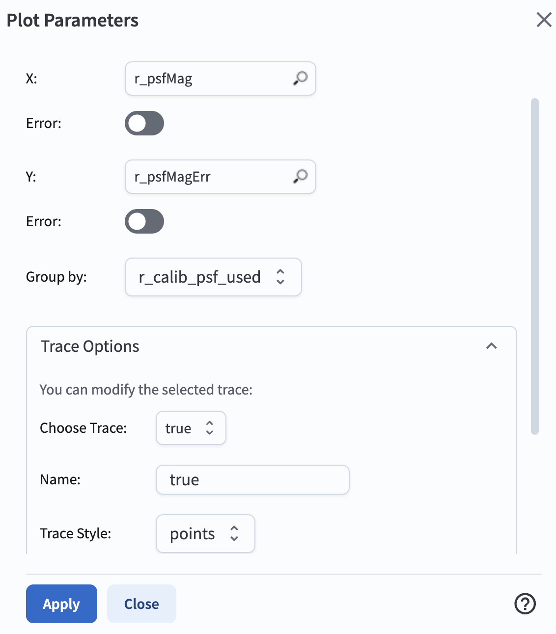
Figure 1: The interface to set plot parameters. It is configured to show r_psfMag on the x-axis and its errors on the y-axis, and to group by the r_calib_psf_used flag.

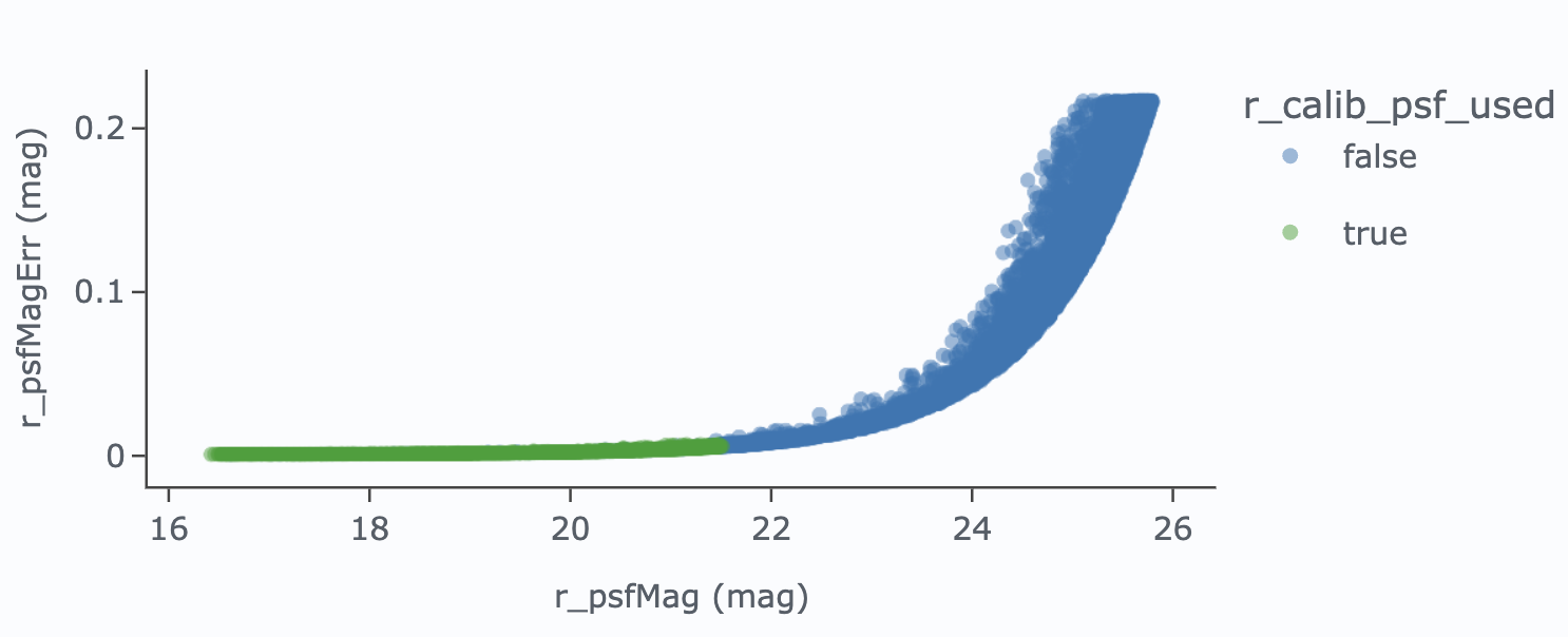
Figure 2: r_psfMagErr vs. r_psfMag for the non-PSF stars (blue circles) and the PSF stars (green circles) in the field. PSF stars are bright and have uncertainties below 1 percent, consistent with the precision achieved by all bright stars.

3. Assess PSF model performance. The LSST Science Pipelines quantify PSF model performance via the object size estimator T (the trace of the second-moment matrix) and the ellipticity components e1 (elongation along the pixel axes) and e2 (elongation along the diagonals). Compute T, e1, e2, and the total ellipticity e for the stars in the table by adding four new columns. Click the “Add a column” icon in the table toolbar (marked with a red box in Figure 3), name the new column T_psf, and enter the expression r_ixxPSF + r_iyyPSF. Repeat this for e1_psf with (r_ixxPSF - r_iyyPSF) / T_psf, for e2_psf with 2 * r_ixyPSF / T_psf, and for e with sqrt(power(e1_psf, 2) + power(e2_psf, 2)).

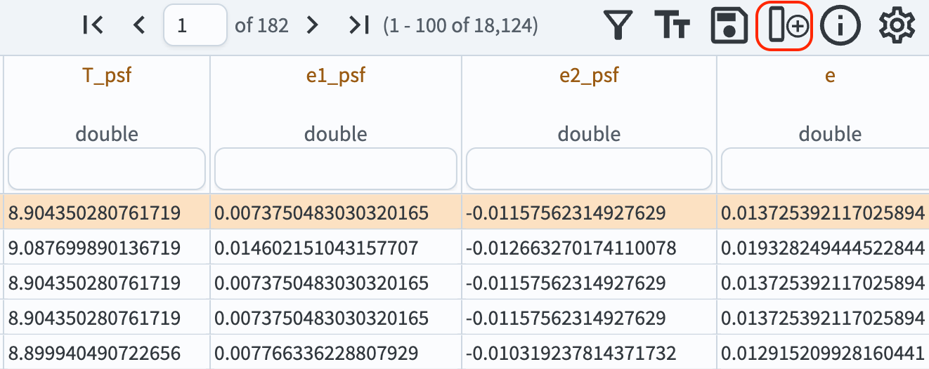
Figure 3: A portion of the results table with four new columns added: T_psf, e1_psf, e2_psf, and e. The “Add a column” icon is marked with a red box.

Add a new chart. Set the plot type to “Histogram”, select T_psf as the column to plot, and click “OK”. Add a second histogram in the same way for the total ellipticity e. To restrict both histograms to the PSF-reserved stars, set the table column condition for r_calib_psf_reserved to “=true”. Delete the scatter plot from Step 2. The two histograms should look like Figure 4.

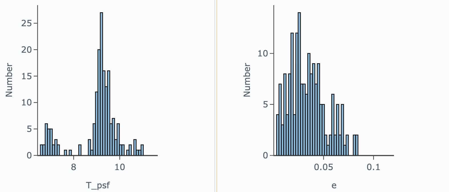
Figure 4: Histograms of the trace of the second-moment matrix, T_psf (left), and the total ellipticity, e (right), for the 181 PSF-reserved stars. The median T ~ 9 pixel² corresponds to a full width at half maximum of about 1 arcsec, given the 0.2 arcsec pixel scale. The ellipticities are small, with most stars below e ~ 0.05, indicating a nearly round PSF model at the positions of the reserved stars.

4. Compare PSF and aperture fluxes. The PSF flux of a point source is aperture corrected to the total calibrated flux, which is tied to a 12-pixel-radius reference aperture, whereas a circular aperture measures only the uncorrected flux enclosed within its radius. In practice, small apertures miss flux, and large apertures admit contamination from neighboring sources and the sky background. This step compares the circular-aperture fluxes (radii of 3 to 70 pixels, centered on the stellar positions) to the PSF fluxes.

Create a new scatter plot of the ratio of PSF flux to the 3-pixel aperture flux as a function of PSF magnitude: set the x-axis to r_psfMag and enter the expression r_psfFlux / r_ap03Flux in the y-axis field. Repeat this for the 12-pixel and 70-pixel apertures (r_ap12Flux and r_ap70Flux). The three plots should look like the panels in Figure 5.

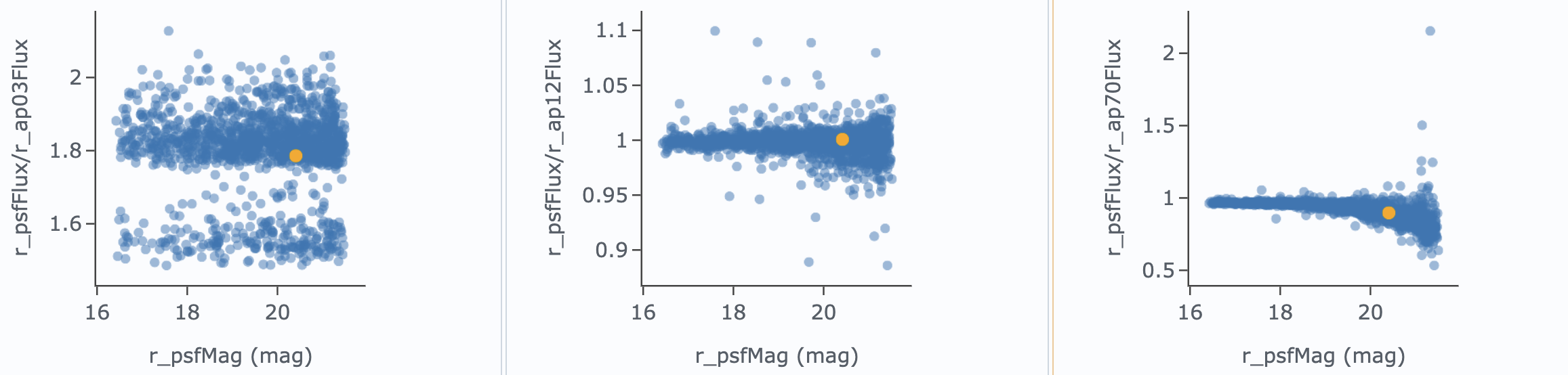
Figure 5: Each panel shows the ratio of PSF flux to aperture flux as a function of PSF magnitude for stars in the field, for aperture radii of 3, 12, and 70 pixels. Ratios > 1 indicate that the aperture is too small to capture the total stellar flux, while ratios < 1 suggest contamination from neighboring sources when the aperture is too large.